
Regression:
Regression analysis stands as the bedrock of predictive modeling, a statistical powerhouse widely employed in data science, economics, and beyond. At its core, regression seeks to illuminate the relationship between variables, allowing us to forecast one based on the others. In this comprehensive guide, we’ll journey through the fundamental components of regression before delving into distinct types, accompanied by real-world examples and practical code implementations.
Key Components:
Dependent Variable (Y):
• Definition: The target variable we aim to predict or explain.
• Significance: Serves as the focal point of the analysis.
Independent Variable(s) (X):
• Definition: Variables utilized to predict the dependent variable.
• Significance: The driving forces behind the predictive power of the model.

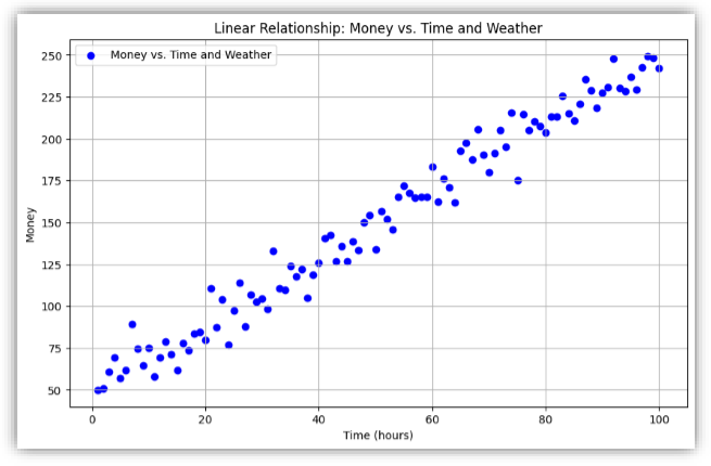
Take the above example the factors such as weather and time are independent variable meaning that independent variables do not rely on anything else. Their values are individualistic and are the cause for the change in the dependent variables. Once again, as the name suggests, independent variables are independent of outside factors. On the other hand, the amount earned by selling the ice-cream is dependent on these variables. As the name suggests, its quantity is dependent on the other. Dependent variables do not change on their own, they change due to other factors.
Linear Relationship:
• Definition: Assumes a linear connection between variables.
• Significance: Simplifies the modeling process, making it more interpretable.
Considering the above example, the linear relationship will look like this
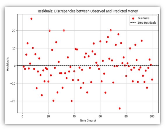
Residuals:
• Definition: The disparities between observed and predicted values.
• Significance: Aid in evaluating the model’s accuracy and identifying areas for improvement.
For the above scenario the residual plot will be
Types of Regression:
• Simple Linear Regression
• Multiple Linear Regression
• Polynomial Regression
• Ridge Regression (L2 Regularization)
• Lasso Regression (L1 Regularization)
Simple Linear Regression
Simple Linear Regression is a statistical method used to model the relationship between a single independent variable (predictor) and a dependent variable. It assumes a linear relationship, aiming to find the
best-fit line that minimizes the sum of squared differences between observed and predicted values.
Use:
Simple Linear Regression is widely employed for predictive analysis and trend identification when there is a belief that one variable influence another in a linear fashion.
Concept: The core concept is expressed in the equation:
Y=b0+b1×X+ε
• Y: Dependent variable
The outcome or response variable that we are trying to predict or explain in a statistical model.
• X: Independent variable
The variable that is being manipulated or controlled in an experiment or study and is used to predict or explain changes in the dependent variable in a statistical model.
• b0: Y-intercept (constant)
The beta zero represents the y-intercept, a constant term in the linear regression equation, indicating the value of the dependent variable when the independent variable is zero.
• b1: Slope (coefficient)
The beta one is the slope coefficient in the linear regression equation, representing the rate of change in the dependent variable for a oneunit change in the independent variable .
• ε: Residuals (errors)
This symbol represents residuals, which are the differences between the observed values of the dependent variable and the values predicted by the regression model. Residuals measure the accuracy of the model, with ideally small and randomly distributed residuals indicating a good fit.
Real-world Example:
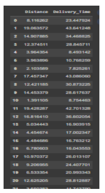
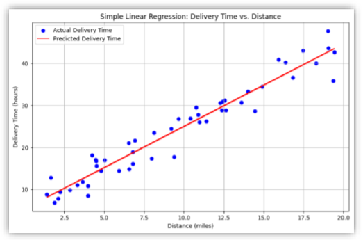
Suppose you are a data scientist working for a delivery company. You hypothesize that the time it takes to deliver a package (Y) is linearly dependent on the distance of the delivery (X). The goal is to predict delivery time based on distance.
Data:
Code:

Output:
- Mean Squared Error (MSE): This measures the average squared difference between the actual and predicted values. Lower MSE indicates better model performance.
- R-squared (Coefficient of Determination): Represents the proportion of the variance in the dependent variable that is predictable from the independent variable. R-squared values range from 0 to 1, where 1 indicates a perfect fit. Higher Rsquared values suggest a better fit.


